Planted Machine Learning
Letting accuracy and interpretability go hand in hand

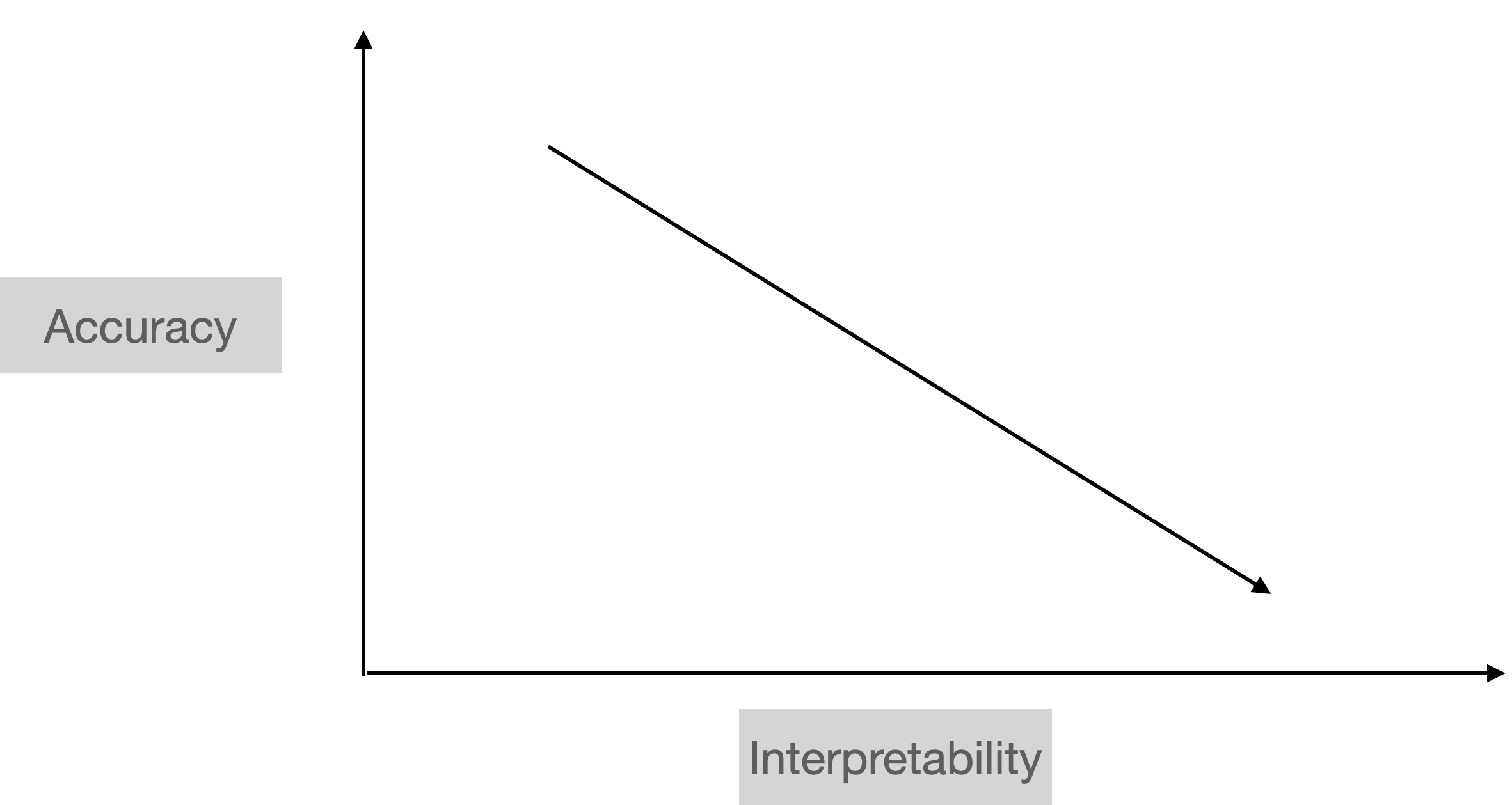
Accuracy vs Interpretability
General Conception
Conjecture: Interpretability can boost accuracy 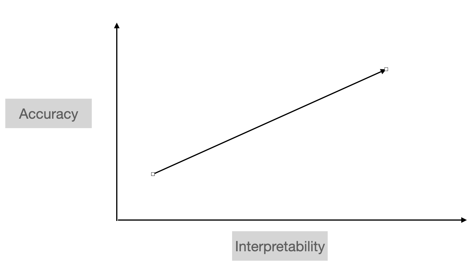
The curse of dimensionality an example
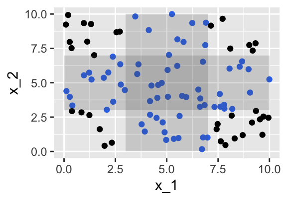
We first generate 100 observations of the \(x_1\) variable which is uniformly distributed on [0,10].
A total of 42 observations are within a distance of 2 units from the middle point 5
We generate \(x_2\) independent of \(x_1\) and uniformly distributed on \([0,10]\).
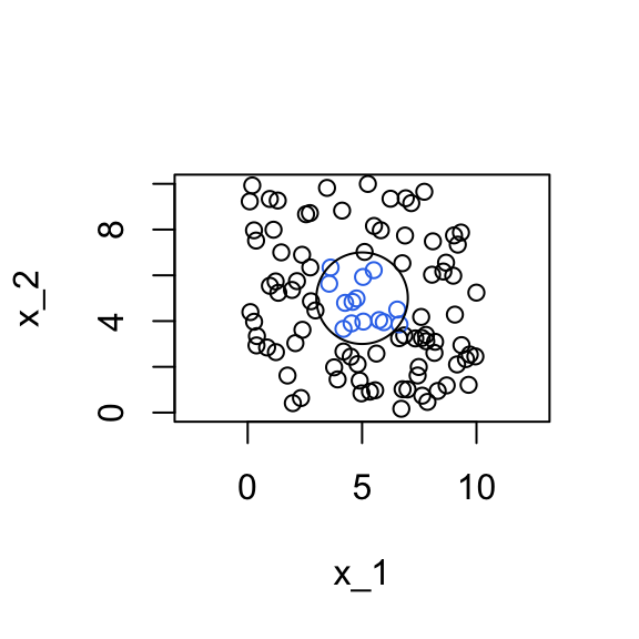
We find 19 observations within a distance of 2 units from the middle point (5,5).
The \(x_3\) variable is independent of \((x_1,x_2)\) and uniformly distributed on \([0,10]\).
Only a total of 9 observation(s) fall within a distance of 2 units from the middle point (5,5,5).
The curse of dimensionality Solutions
There are two ways to tackle the curse of dimensionality
1. Sparsity
Assume that the intrinsic dimension is lower
- E.g. Not all variables are relevant
- Or feature engineer a few highly predictive variables
2. Structure
Interactions are limited and structure can be exploited
- e.g. an additive structure \(m(x)=m_1(x_1)+m_2(x_2)\).

Interpretability
Structure is also essential for interpretability but current machine learning algorithms for tabular data do not make use of structure.
Random Planted Forest
This is joint work with
-

Joseph Meyer
Heidelberg University -

Enno Mammen
Heidelberg University
Preprint is available on https://arxiv.org/abs/2012.14563
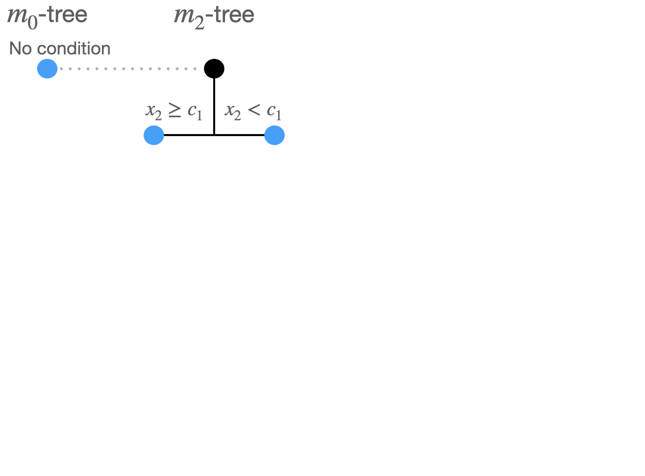
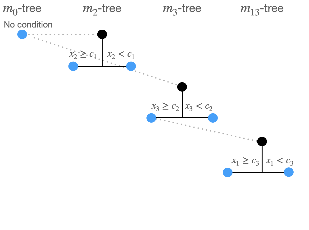
Random Planted Forest The algorithm
Setting: \(dim\)=3, \(t_{try}\)=0.6, \(split_{try}\)=5, \(n_{splits}\)=10
Split 1:
3 possible combinations:
- \(m_0 \rightarrow m_1: x_1\)
- \(m_0\rightarrow m_2: x_2\)
- \(m_0\rightarrow m_3: x_3\)
\(t_{try}:\) \(0.6\times3=1.8 \rightarrow\) 2 viable combinations randomly picked, say:
- \(m_0 \rightarrow m_1: x_1\),
- \(m_0\rightarrow m_2: x_2\)
\(split_{try}:\)For each viable split option we consider 5 randomly picked split points \(\rightarrow\) \(2\times5=10\) split options.
Compare the 10 split options: \(\sum_i (\widehat m(X_i) -Y_i)^2\)
\((m_2tree\rightarrow x_2,c_1)\) produces minimal least squares loss.
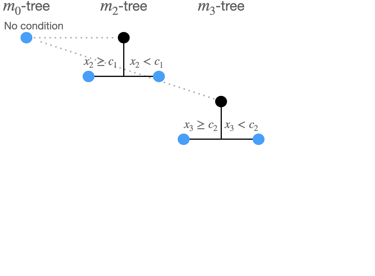
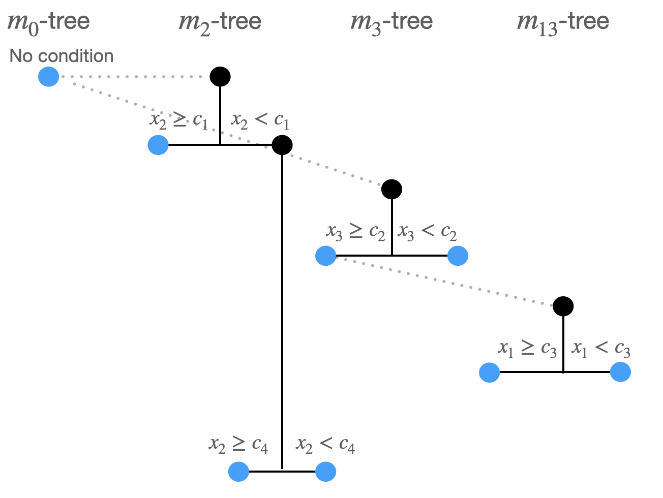
Random Planted Forest The algorithm
Setting: \(dim\)=3, \(t_{try}\)=0.6, \(split_{try}\)=5, \(n_{splits}\)=10
Split 2:
Now: 5 possible split combinations:
- \(m_0 \rightarrow m_1: x_1\)
- \(m_0 \rightarrow m_3: x_3\)
- \(m_2\rightarrow m_{12}: x_1\)
- \(m_2\rightarrow m_{13}: x_3\)
- \(m_2: x_2\)
Viable split combinations: \(5\times0.6=3\) –> 3 options randomly picked, say
- \(m_0\rightarrow m_1: x_1\)
- \(m_2\rightarrow m_{23}: x_3\)
- \(m_0 \rightarrow m_3: x_3\)
Hence \(5\)\(\times(1+2+1)=20\) split options.
\((m_0 \rightarrow m_3: x_3,c_2)\) produces minimal least squares loss.
Random Planted Forest The algorithm
Setting: \(dim\)=3, \(t_{try}\)=0.6, \(split_{try}\)=5, \(n_{splits}\)=10
Split 3:
- Now: 7 possible split combinations:
- \(m_0 \rightarrow m_1: x_1\)
- \(m_2 \rightarrow m_{12}: x_1\)
- \(m_2 \rightarrow m_{13}: x_3\)
- \(m_2 \rightarrow x_2\)
- \(m_3 \rightarrow m_{13}: x_1\)
- \(m_3 \rightarrow m_{23}: x_2\)
- \(m_3 \rightarrow x_3\)
- …
- \((m_3 \rightarrow m_{13}: x_1,c_3)\) produces minimal least squares loss.
Random Planted Forest The algorithm
Setting: \(dim\)=3, \(t_{try}\)=0.6, \(split_{try}\)=5, \(n_{splits}\)=10
Split 4:
- \((m_2 \rightarrow m_{2}: x_2,c_4)\) produces minimal least squares loss.
Random Planted Forest Accuracy: Simulation
Additive, Sparse (2/30 features), Non-linear (sin-curve)

True function: black solid line
Grey lines: 40 Monte Carlo simulations
xgboost (additive=depth=1)
planted forest (additive= max interaction=1)
Simulations are run with optimal parameters
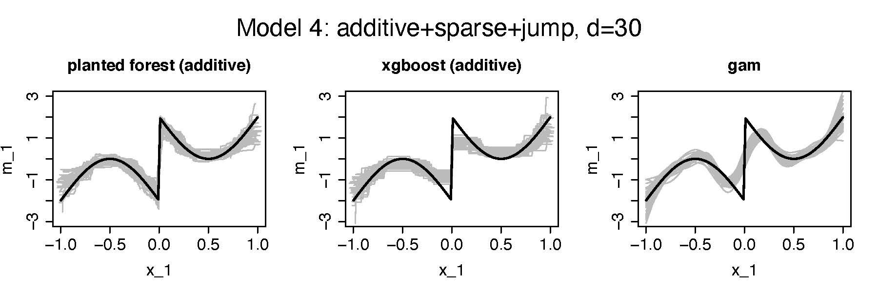
Random Planted Forest Accuracy: Simulation
Second setting:Additive, Sparse (2/30 features), jump
Random Planted Forest Accuracy: Simulation
Third setting:\(\textbf{pair-wise interaction}\), Sparse (2/30 features), smooth
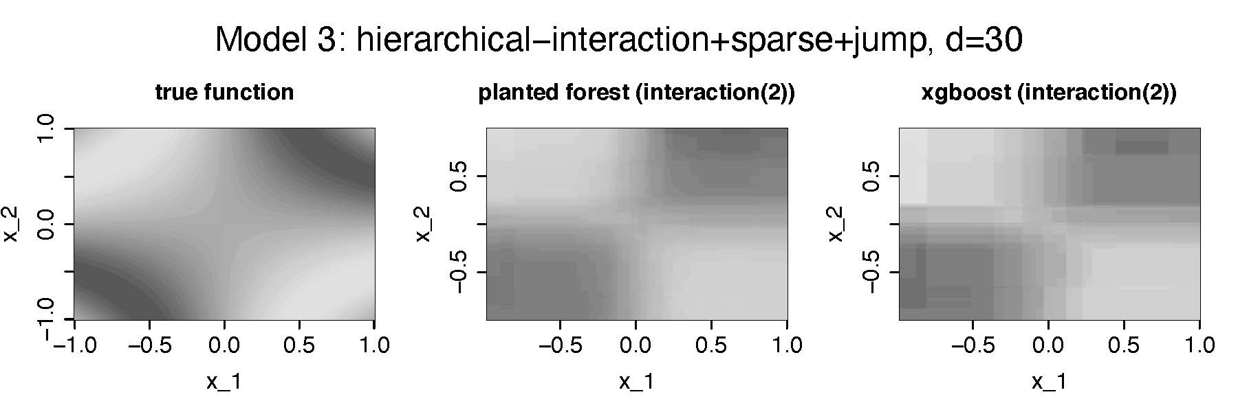
- Estimating \(m_{12}(x_{1},x_2)\)
- We do not consider gam anymore-
- Heatmaps show median performing estimators out of 40 Monte Carlo simulations
Generalized Random Planted Forest
This is joint work with
-
Joseph Meyer
Heidelberg University -
Enno Mammen
Heidelberg University -

Lukas Burk
The Leibniz Institute for Prevention
Research and Epidemiology - BIP -

Marvin Wright
The Leibniz Institute for Prevention
Research and Epidemiology - BIP
Code is available on https://github.com/PlantedML/randomPlantedForest
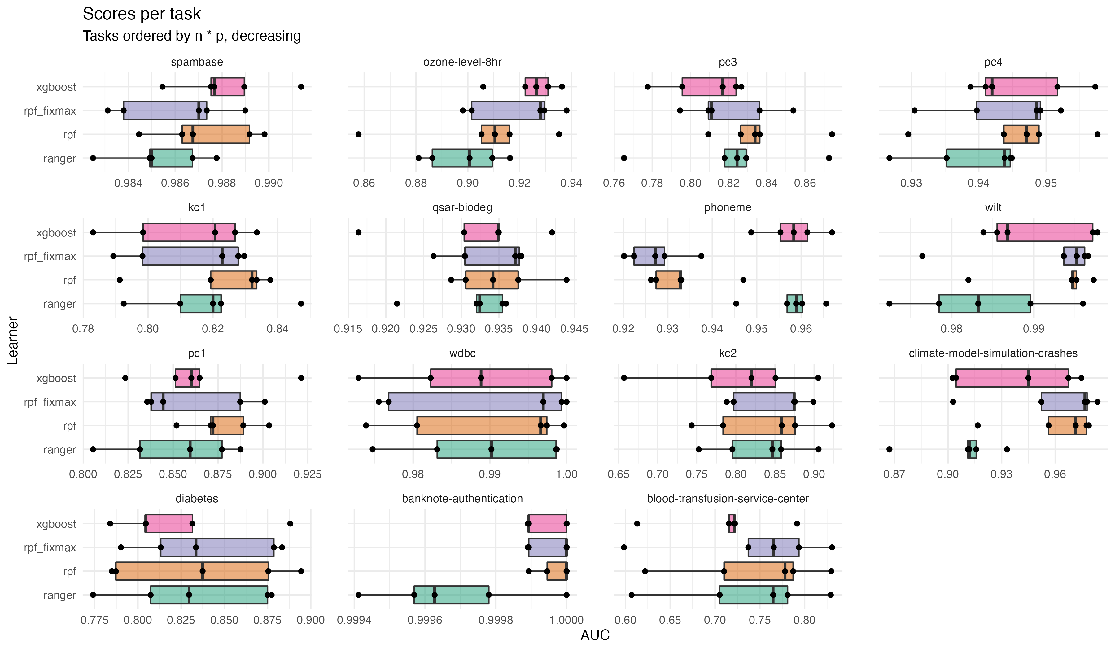
Random Planted Forest Accuracy: Benchmark-data
Interpretability
This is joint work with
-
Joseph Meyer
Heidelberg University -
Marvin Wright
The Leibniz Institute for Prevention
Research and Epidemiology - BIP
Preprint is available on https://arxiv.org/abs/2208.06151
Code is available on https://github.com/PlantedML/glex
Interpretability Marginal Identification: fairness
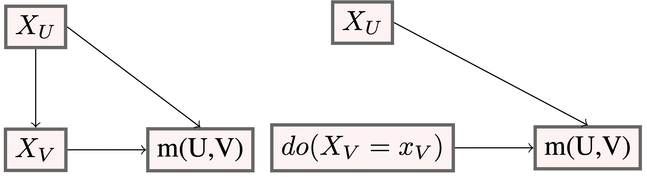
Assume \(U\) is a set of protected features.
- For example \(U=\{\text{gender, ethnicity}\}\).
Let \(U \cup V=\{1,\dots, d\}, U\cap V=\emptyset\).
The do-operator, \(do(X_V=x_V)\), removes all edges going into \(X_V\), ensuring counterfactual fairness (Kusner et al. 2017), see also Lindholm et al. (2022)
\(E[m(X) |\ do(X_V=x_V))\) does not use information contained in \(X_U\); neither directly nor indirectly.
Under the assumed causal structure we have \[E[m(X) |\ do(X_V=x_V)]= \int m(x) p_U(x_U) dx_U.\]
Under marginal identifiaction: \[\int \hat m^\ast(x) \hat p_U(x_U) dx_U= \sum_{S: S\cap U =\emptyset}\int \hat m^\ast_S(x_S) \hat p_U(x_U) dx_U + \sum_{S: S\cap U \neq \emptyset}\int \hat m^\ast_S(x_S) \hat p_U(x_U) dx_U= \sum_{S \subseteq V} \hat m^\ast_S(x_S),\] i.e., a “fair” estimator can be extracted from \(\hat m\) by dropping all components that include features in \(U\).
Interpretability Marginal Identification:Simulation
We simulate 10,000 noisy observations from
\[m(x_1,x_2)=x_1+x_2+x_1x_2\] If \(X_1, X_2\) have each mean zero and variance one, then
- Marginal identification: \[ \begin{eqnarray} m_0&=&2corr(X_1,X_2) \\ m_1(x_1)&=& x_1 -2corr(X_1,X_2) \\ m_2(x_2)&=&x_2 - 2corr(X_1,X_2) \\ m_{12}(x_1,x_2)&=& 2x_1x_2 + 2corr(X_1,X_2). \end{eqnarray} \]
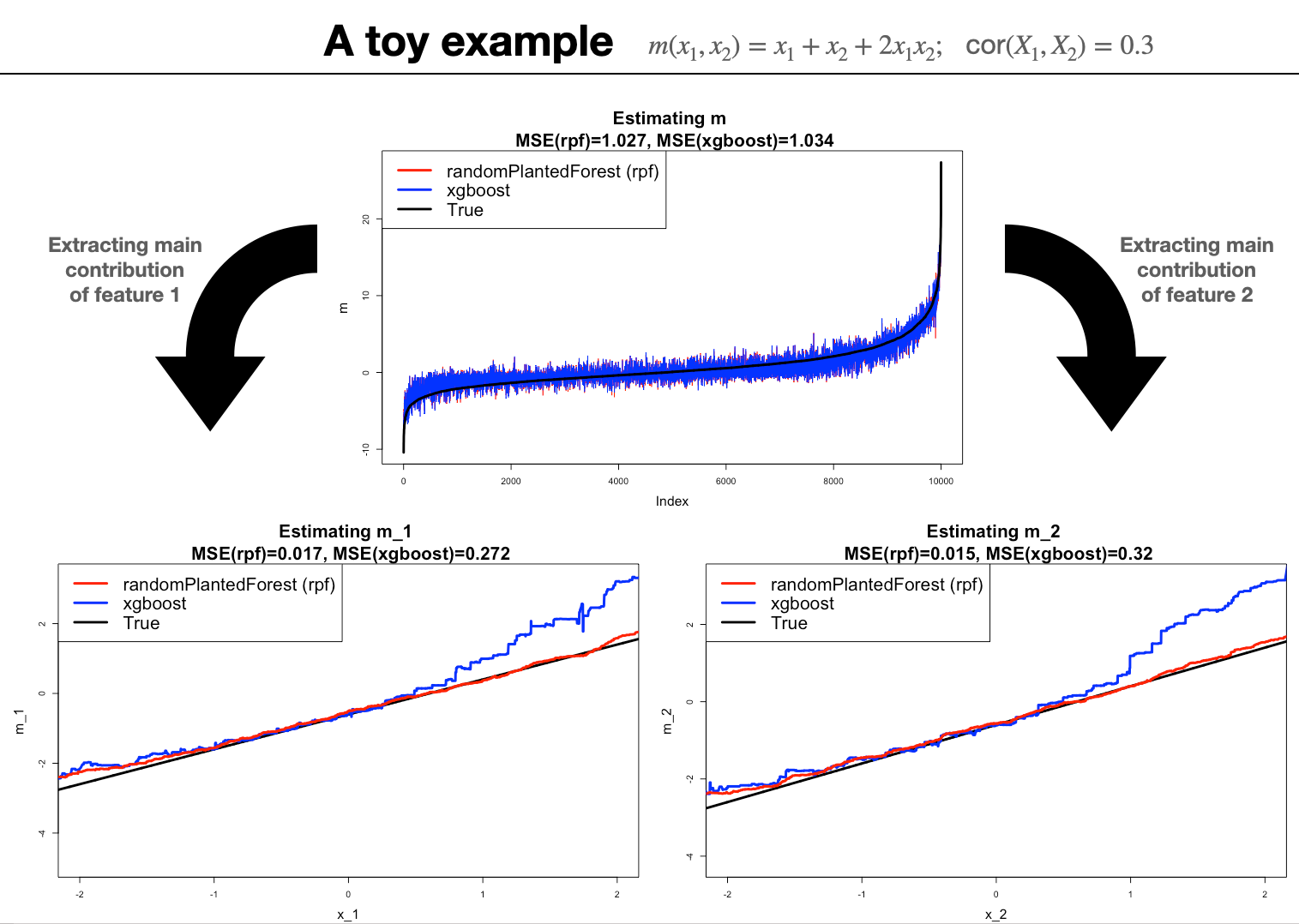
- Conclusion: It is not clear if a method that estimates \(m\) well is also a good estimator for a selection of components {\(m_S\)}.
- This discussion is related to work done in double/debiased machine learning Chernozhukov et al. (2018).